Advanced D3: Layouts and Maps

Material based on Scott Murray’s book and blocks by Mike Bostock

Layouts

Layouts make it easier to lay elements representing your data out on the screen. While we’ve produced layouts ourselves already, we’ve only used simple position and size assignments that were directly driven by the data. In this lecture we will learn how to use D3’s layout features to produce more complex layouts.

Layouts don’t actually draw things for us, rather they perform a data transformation that we can use to draw specific objects on the screen. Let’s start with a simple example, a pie chart.

A Pie Chart

Pie charts are not a very good visaulization technique, they have multiple weaknesses compared to their alternatives. We’ll talk about those in class, but for now, we’ll draw a pie chart because it’s one of the simplest layouts we can do.

In the following example, we use the D3 pie layout to calculate the angles and the D3.svg.arc function to calculate the arcs used for drawing the wedges.

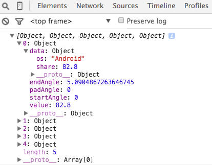The interesting intermediate stages here are the values produced by the pie layout and the path drawn by the arc function. The pie layout produces a specific data object that we can use to bind to the DOM elements, shown on the right. We ge an array with one ojbect for each wedge. The first member of the object is data, which stores the raw data. We also have startAngel and endAngle (in radians).

The path that is generated by the arc function, is the second piece of information: M1.1634144591899855e-14,-190A190,190 0 1,1 -176.58002257840997,-70.13911623486732L0,0Z. This defines the actual path drawn.

A Force-Directed Graph Layout

We’ve mainly talked about tabluar data up to this point. As we will soon learn, there are other data forms. A major other data form is the graph or network. Graphs describe relations between elements. The elements are usually referred to as nodes or vertices, the relationships as links or edges. A common, but not the only representation for graphs are node link diagrams, where nodes are often rendered as circles and edges as lines connecting the circles. There are many ways to lay the nodes in a graph out. We could have all nodes on a circle, or in a grid, or use some other method for laying them out. A common method is a force-directed layout. The idea behind a force directed layout is a physical model: the nodes repulse each other, while the edges are considered springs that pull each other close. The idea behind this is that as nodes that are tightly connected will be close to each other, i.e., form visible clusters, whereas nodes that are not connected are far from each other. The D3 implementation does not actually model this as springs, but as geometric constraints, but the mental model is still useful.

This happens in an iterative process, i.e., the forces for each node to each other node are calculated in a single step and the system is adjusted, then the next loop starts, etc. Eventually, the system will (hopefully) find an equilibrium. This is computationally expensive, as we will learn, but works fine for smaller graphs.

The following example illustrates a node-link diagram based on character co-occurrences in Les Miserables. It is based on the standard D3 force layout example.

The data is stored in a json file. Here is a sample of this file:

 1 {
 2   "nodes":[
 3     {"name":"Myriel","group":1},
 4     {"name":"Napoleon","group":1},
 5     {"name":"Mlle.Baptistine","group":1},
 6     {"name":"Mme.Magloire","group":1},
 7     {"name":"CountessdeLo","group":1}
 8   ],
 9   "links":[
10     {"source":1,"target":0,"value":1}
11     {"source":2,"target":0,"value":8},
12     {"source":3,"target":0,"value":10},
13     {"source":3,"target":2,"value":6},
14     {"source":4,"target":0,"value":1}
15   ]
16 }

The file contains a list of nodes, followed by a list of edges (links), a common format to store graph data. In the array of nodes, we have objects with the values name and group, the links array contain the edges that are defined via a source and target, which are indices into the nodes array (e.g., source 1 is Napoleon, traget 0 is Myriel).

First we will used D3’s XMLHttpRequest module (XHR), specifically the JSON method to load the data. Two things are important to note:

1. Once the data is loaded it will be available in an object, just as we see it in the json file.
2. The XMLHttpRequest methods load asynchronously. That means that we’ll not get a return value from the loading function right away, but rather pass a function that is executed when the data loading is complete. The benefit of the asynchronous function is, of course, that other processes can continue, e.g., a user interface wouldn’t freeze up while a dataset is loaded.

We then use the force layout to calculate the initial positions and update them in “ticks”:

The layout uses a “cooling” factor that stops the iteration cycle.

Other Layouts

There are many other layouts that can be very valuable, for. We’ll revisit the layouts in class when we talk about the specific techniques they implement, but the principle is always the same: they take data and calculate derived data, which you then can use to position/scale graphical primitives on the canvas. You shouldn’t have a hard time understanding any of the other layout examples.

Maps

Maps, finally! But before we start talking about how to draw maps, a word of caution: maps are heavily over-used. A lot of information that is printed on top of maps would be better of in another type of chart. If we compare data of the five largest cities in the US, we don’t need to do that on a map, everyone knows where New York, Los Angeles, Chicago, Houston, and Philadelphia are, but if we plot this on a map we give up our most important visual channel: position. We’re no longer free to place things where we want!

But let’s get to how we do maps with D3. Generally, there are two approaches:

1. Street Map with Data: If you want to show something in the context of a real street map, your best bet is to use something like the Google Maps API - here’s an example of how it’s used with D3, or the OpenStreetMap API. You can use D3 to draw things on top of those, but you’ll mainly work with the API provided by the vendor.
2. Data Maps: If you want to present data on an abstract map, e.g., only showing counties or state borders, D3 is the way to go! We’ll be taking about data maps from now on.

D3 Maps are based on the GeoJSON format (or the TopoJSON variety). The GeoJSON format describes the contained geography as a combination of longitude and latitude coordinates, so that each entry forms a polygon. Here is a sample from the data file containing US states.

 1 {
 2      "type":  "FeatureCollection",
 3      "features":
 4      [
 5          {
 6              "type": "Feature",
 7              "id": "01",
 8              "properties": {"name": "Alabama"},
 9              "geometry": {
10                 "type": "Polygon", 
11                 "coordinates": [[[-87.359296, 35.00118], [-85.606675, 34.984749], [-85.431413,34.124869],[-85.184951,32.859696], ... 
12  }

You can see that the coordinates are within the geometry object, and that the properties tell us that this is the shape repesenting Alabama. These polygons can be easily converted into an SVG path with d3.geo.path() (as always, see the API documentation here).

The previous map uses the geographical information with a default projection. Projections are necessary because the earth is a sphere and can not be directly depicted, without a projection, on a flat surface. There are many projections, with various advantages and disadvantages - we’ll talk about them in class. Let’s center the map and try out a couple:

There are a lot of map projections implemented in D3. Here is a showreel.

Here is an example for a choropleth map, coloring each state by its agricultural output. The trick here is to join the data about the ouptut to the geography information:

Here is an example for how we can draw marks on top of maps, in this case the size of cities:

Next Steps

This concludes our introduction to D3 and JavaScript. We will (probably) have another lecture on designing larger systems, event handling, etc in the next couple of weeks.