
Advanced D3: Layouts
Material based on Scott Murray’s book and blocks by Mike Bostock
Layouts
Layouts make it easier to spatially arrange, shape and size elements representing data on the screen. While we’ve produced layouts ourselves already, we’ve only used simple position and size assignments that were directly driven by the data. And while these cover important classes of visualization techniques, there are more advanced techniques for different data types that are not as easily placed. Layouts are typically based on algorithms that define, e.g., where to put a node in a network visualization, or where to place a rectangle in a tree map. In this lecture we will learn how to use D3’s layout features to render such complex layouts.
D3 Layouts don’t actually draw things for us, rather they perform a data transformation that we can use to draw specific objects on the screen. Let’s start with a simple example, a pie chart.
Pie/Donut Charts
Pie charts are a much criticised visualization technique as they have multiple weaknesses (but also strengths) compared to their alternatives. We’ll talk about those in class, but for now, we’ll draw a pie chart because it’s one of the simplest layouts we can do.
Let us consider the following line of code: pie = d3.pie(data). It is important to note that the d3.pie() call does not produce a shape directly, but computes the necessary angles to represent a dataset as a pie or donut chart.
The data output by d3.pie(data) can then be used as follows: arc = d3.arc(pie).
Here, d3.arc() (the arc generator) produces a circular svg shape, as in a pie or donut chart.
Let’s take a closer look at the output of d3.pie(data).
- data - element
- index - of the element
- value - of the arc.
- startAngle - of the arc. The overall start angle of the pie, i.e., the start angle of the first arc.
- endAngle - The overall end angle of the pie, i.e., the end angle of the last arc
- padAngle - of the arc. The pad angle here means the angular separation between each adjacent arc.
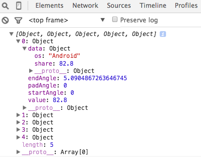 The interesting intermediate stages here are the values produced by the pie layout and the path drawn by the arc function. The pie layout produces a specific data object that we can use to bind to the DOM elements, shown on the right. We get an array with one object for each wedge. The first member of the object is
 data, which stores the raw data. We also have startAngle and endAngle (in radians).
The path that is generated by the arc function, is the second piece of information: M1.1634144591899855e-14,-190A190,190 0 1,1 -176.58002257840997,-70.13911623486732L0,0Z. This defines the actual path drawn.
Hierarchy Layouts
Chord Layout
Chord diagrams are often used to show directed relationships among a group of entities. d3.chord() computes the chord layout for the specified square matrix of size n×n, where the matrix represents the directed flow amongst a network of n nodes. The given matrix must be an array of length n, where each element matrix[i] is an array of n numbers, where each matrix[i][j] represents the flow from the ith node in the network to the jth node. Each number matrix[i][j] must be nonnegative, though it can be zero if there is no flow from node i to node j.
Here is an example dataset:
var matrix = [
  [11975,  5871, 8916, 2868],
  [ 1951, 10048, 2060, 6171],
  [ 8010, 16145, 8090, 8045],
  [ 1013,   990,  940, 6907]
];
We will look at 3 d3 functions in order to render a complete chord diagram.
- d3.chord() - analagous to d3.pie() in our previous example, returns the data formatted properly for our svg path generator.
- d3.arc() - path generator for the outside circle
- d3.ribbon() - path generator for the inside ribbons
The return value of d3.chord(matrix) is an array of chords, where each chord represents the combined bidirectional flow between two nodes i and j (where i may be equal to j) and is an object with the following properties:
- source - the source subgroup
- target - the target subgroup
Each source and target subgroup is also an object with the following properties:
- startAngle - the start angle in radians
- endAngle - the end angle in radians
- value - the flow value matrix[i][j]
- index - the node index i
- subindex - the node index j
The chords are typically passed to d3.ribbon to display the network relationships.
The chords array also defines a secondary array of length n, chords.groups, where each group represents the combined outflow for node i, corresponding to the elements matrix[i][0 … n - 1], and is an object with the following properties:
- startAngle - the start angle in radians
- endAngle - the end angle in radians
- value - the total outgoing flow value for node i
- index - the node index i
The groups are typically passed to d3.arc to produce a donut chart around the circumference of the chord layout.
Let’s step through a simple example to see how this works. Notice that our final chord diagram has two types of svg paths. The arcs that form the outer layer and the ribbons that form the connecting chords.
See output in new page.Let’s wrap up Chord Diagrams with this look at a really creative use of a Chord Diagram Lord of the Rings Chord Diagram
Tree Layout
Let’s talk about trees, a very common layout for hierarchical data.
d3.tree() Creates a new tree layout with default settings.
However, before we can compute a hierarchical layout, we need a root node. If our data is already in a hierarchical format, such as JSON, we can pass it directly to d3.hierarchy; otherwise, we can rearrange tabular data, such as comma-separated values (CSV), into a hierarchy using d3.stratify.
Let’s assume with have this data:
{
  "name": "Eve",
  "children": [
    {
      "name": "Cain"
    },
    {
      "name": "Seth",
      "children": [
        {
          "name": "Enos"
        },
        {
          "name": "Noam"
        }
      ]
    },
    {
      "name": "Abel"
    },
    {
      "name": "Awan",
      "children": [
        {
          "name": "Enoch"
        }
      ]
    },
    {
      "name": "Azura"
    }
  ]
}
We can now call d3.hierarchy on this data as such:
let root = d3.hierarchy(data[, children])
If we are provided the data in a non-hierarchical format, as if loaded a CSV file:
[
  {"name": "Eve",   "parent": ""},
  {"name": "Cain",  "parent": "Eve"},
  {"name": "Seth",  "parent": "Eve"},
  {"name": "Enos",  "parent": "Seth"},
  {"name": "Noam",  "parent": "Seth"},
  {"name": "Abel",  "parent": "Eve"},
  {"name": "Awan",  "parent": "Eve"},
  {"name": "Enoch", "parent": "Awan"},
  {"name": "Azura", "parent": "Eve"}
]
Then we need to wrangle this data into a hierarchy.
This is where d3.stratify comes in. d3.stratify()(data) generates a new hierarchy from the specified tabular data:
let stratify = d3.stratify()
    .id(d => d.name)
    .parentId(d => d.parent);

let root =  stratify(data);
Both d3.hierarchy and d3.stratify should return a root node that looks like:
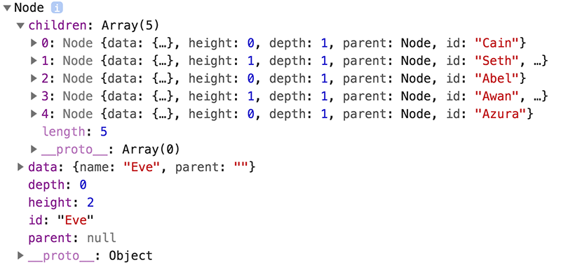
This returned root node and each descendant has the following properties:
- node.data - the associated data, as specified to the constructor.
- node.depth - zero for the root node, and increasing by one for each descendant generation.
- node.height - zero for leaf nodes, and the greatest distance from any descendant leaf for internal nodes.
- node.parent - the parent node, or null for the root node.
- node.children - an array of child nodes, if any; undefined for leaf nodes.
- node.value - the summed value of the node and its descendants; optional, see node.sum and node.count.
The node objects also have two functions that will prove useful in this context:
-
node.ancestors() - Returns the array of ancestors nodes, starting with this node, then followed by each parent up to the root.
-
node.descendants() - Returns the array of descendant nodes, starting with this node, then followed by each child in topological order.
Once we have our root node, we can feed it into the tree layout.
d3.tree(root) lays out the specified root hierarchy, assigning the following properties on root and its descendants and assigns a x and y coordinate to each node.
- node.x - the x-coordinate of the node
- node.y - the y-coordinate of the node
Treemap Layout
Introduced by Ben Shneiderman in 1991, a treemap recursively subdivides area into rectangles according to each node’s associated value.
This example is based on this block
For the Treemap layout we will be looking at how to convert tabular data in csv form to the final layout.
Let’s consider our input data, which looks something like this:
size,path
90,d3/d3-array/array.js
86,d3/d3-array/ascending.js
238,d3/d3-array/bisect.js
786,d3/d3-array/bisector.js
72,d3/d3-array/constant.js
86,d3/d3-array/descending.js
Because our final layout is meant to represent hierarchical data, we must first wrangle this table into a hierarchy using d3.stratify. Once we have our root, we can then use d3.treemap() to get our layout/positions:
d3.treemap() - Creates a new treemap layout with default settings.
treemap(root) - Lays out the specified root hierarchy, assigning the following properties on root and its descendants:
- node.x0 - the left edge of the rectangle
- node.y0 - the top edge of the rectangle
- node.x1 - the right edge of the rectangle
- node.y1 - the bottom edge of the rectangle
Note that you must call root.sum before passing the hierarchy to the treemap layout. You probably also want to call root.sort to order the hierarchy before computing the layout. Any ideas why?
See output in new page.Network Layouts
Node Link Force-Directed Graph Layout
We’ve mainly talked about tabluar data up to this point. As we will soon learn, there are other data forms. A major other data form is the graph or network. Graphs describe relations between elements. The elements are usually referred to as nodes or vertices, the relationships as links or edges. A common, but not the only representation for graphs are node link diagrams, where nodes are often rendered as circles and edges as lines connecting the circles. There are many ways to lay the nodes in a graph out. We could have all nodes on a circle, or in a grid, or use some other method for laying them out. A common method is a force-directed layout. The idea behind a force directed layout is a physical model: the nodes repulse each other, while the edges are considered springs that pull each other close. The idea behind this is that as nodes that are tightly connected will be close to each other, i.e., form visible clusters, whereas nodes that are not connected are far from each other. The D3 implementation does not actually model this as springs, but as geometric constraints, but the mental model is still useful.
This happens in an iterative process, i.e., the forces for each node to each other node are calculated in a single step and the system is adjusted, then the next loop starts, etc. Eventually, the system will (hopefully) find an equilibrium. This is computationally expensive, as we will learn, but works fine for smaller graphs.
The following example illustrates a node-link diagram based on character co-occurrences in Les Miserables. It is based on the standard D3 force layout example.
The data is stored in a json file. Here is a sample of this file:
1
2
3
4
5
6
7
8
9
10
11
12
13
14
15
16
17
{
  "nodes":[
    {"id":"Myriel","group":1},
    {"id":"Napoleon","group":1},
    {"id":"Mlle.Baptistine","group":1},
    {"id":"Mme.Magloire","group":1},
    {"id":"CountessdeLo","group":1}
  ],
  "links":[
    {"source": "Napoleon", "target": "Myriel", "value": 1},
    {"source": "Mlle.Baptistine", "target": "Myriel", "value": 8},
    {"source": "Mme.Magloire", "target": "Myriel", "value": 10},
    {"source": "Mme.Magloire", "target": "Mlle.Baptistine", "value": 6},
    {"source": "CountessdeLo", "target": "Myriel", "value": 1}

  ]
}
The file contains a list of nodes, followed by a list of edges (links), a common format to store graph data. In the array of nodes, we have objects with the values id and group, the links array contain the edges that are defined via a source and target, which are the ids of the source and target nodes respectively).
First we will used D3’s d3-fetch module, specifically the JSON method to load the data. Two things are important to note:
- Once the data is loaded it will be available in an object, just as we see it in the json file.
- The d3-request methods load asynchronously. That means that we’ll not get a return value from the loading function right away, but rather pass a function that is executed when the data loading is complete. The benefit of the asynchronous function is, of course, that other processes can continue, e.g., a user interface wouldn’t freeze up while a dataset is loaded.
We then use the force layout to calculate the initial positions and update them in “ticks”:
Forces
A force is simply a function that can be used to modify nodes’ positions or velocities. A force can apply a classical physical force such as electrical charge or gravity, or it can resolve a geometric constraint, such as keeping nodes within a bounding box or keeping linked nodes a fixed distance apart.
Possible forces include:
- Links
- Many-Body
- Centering
- Collision
- Positioning
Here is how you would start a new simulation with a specifie array of nodes and no forces. If nodes is not specified, it defaults to the empty array.
var simulation = d3.forceSimulation();
In order to add forces, we use the .force syntax as such:
simulation
     .force("link", d3.forceLink().id(d => d.id))
     .force("charge", d3.forceManyBody())
     .force("center", d3.forceCenter(width / 2, height / 2));
These happen to be the three forces that are at play in the example we will look through below. In order to understand their effect, let’s take a look at what happens when we remove each one.
forceLink()
The link force pushes linked nodes together or apart according to the desired link distance. When we remove it, there is nothing keeping the nodes together.
simulation
     .force("charge", d3.forceManyBody())
     .force("center", d3.forceCenter(width / 2, height / 2));
The syntax for forceLink() is as follows:
d3.forceLink().id(d => d.id))
If id is specified, sets the node id accessor to the specified function and returns this force.
If id is not specified, returns the current node id accessor, which defaults to the numeric index of the node:
function id(d, i) {
  return i;
}
forceManyBody()
The many-body force applies mutually amongst all nodes. It can be used to simulate gravity (attraction) if the strength is positive, or electrostatic charge (repulsion) if the strength is negative.
You can set the strength of this force with d3.forceManyBody().strength([strength]). If strength is not specified, returns the current strength accessor, which defaults to -30.
simulation
     .force("link", d3.forceLink().id(d => d.id))
     .force("center", d3.forceCenter(width / 2, height / 2));
forceCenter()
The centering force translates nodes uniformly so that the mean position of all nodes is at the given position ⟨x,y⟩
simulation
     .force("link", d3.forceLink().id(d => d.id))
     .force("charge", d3.forceManyBody())
forceCollide()
The collision force treats nodes as circles with a given radius, rather than points, and prevents nodes from overlapping
simulation
     .force("collide", d3.forceCollide([50])
d3.forceX([X]) / d3.forceY([y])
The x- and y- positioning forces push nodes towards a desired position along the given dimension with a configurable strength.
To fix a node in a given position, specify: fx - the node’s fixed x-position fy - the node’s fixed y-position
Rendering the Simulation
So we’ve created a simulation and added forces, now we assign nodes to the simulation:
simulation
     .nodes(graph.nodes)
Each node must be an object. The following properties are assigned by the simulation:
- index - the node’s zero-based index into nodes
- x - the node’s current x-position
- y - the node’s current y-position
- vx - the node’s current x-velocity
- vy - the node’s current y-velocity
If we used the forceLink() force, we must assign the actual link data to this force:
 simulation.force("link")
       .links(graph.links);
Each link is an object with the following properties:
- source - the link’s source node;
- target - the link’s target node;
- index - the zero-based index into links, assigned by this method
Let’s check out a complete example:
See output in new page.The layout uses a “cooling” factor that stops the iteration cycle.
And to wrap up d3 layouts a cool example using custom made forces!
Cytoscape.js
Cytoscape.js is an open-source graph theory (a.k.a. network) library written in JS. You can use Cytoscape.js for graph analysis and visualisation.
Cytoscape.js allows you to easily display and manipulate rich, interactive graphs. Because Cytoscape.js allows the user to interact with the graph and the library allows the client to hook into user events, Cytoscape.js is easily integrated into your app, especially since Cytoscape.js supports both desktop browsers, like Chrome, and mobile browsers, like on the iPad. Cytoscape.js includes all the gestures you would expect out-of-the-box, including pinch-to-zoom, box selection, panning, et cetera.
Cytoscape.js also has graph analysis in mind: The library contains many useful functions in graph theory. You can use Cytoscape.js headlessly on Node.js to do graph analysis in the terminal or on a web server.
A complete example is given below:
See output in new page.Other Layouts
There are many other layouts that can be very valuable, for. We’ll revisit the layouts in class when we talk about the specific techniques they implement, but the principle is always the same: they take data and calculate derived data, which you then can use to position/scale graphical primitives on the canvas. You shouldn’t have a hard time understanding any of the other layout examples.