Maps

Before we start talking about how to draw maps, a word of caution: maps are heavily over-used. A lot of information that is printed on top of maps would be better shown in another type of chart. If we compare data of the five largest cities in the US, we don’t need to do that on a map, everyone knows where New York, Los Angeles, Chicago, Houston, and Philadelphia are, but if we plot this on a map we give up our most important visual channel: position. We’re no longer free to place things where we want!

There are, however, cases, when the spatial position is paramount, and in this case you should definitely use a map.

But let’s get to how we can visualize data on top of maps with D3. Generally, there are two approaches:

1. Data Maps: If you want to present data on an abstract map, e.g., only showing counties or state borders, D3 is the way to go! Data maps are mostly used for when you want to communicate trends and let users compare between different areas. In these maps you have full control over how the map is colored, and how to encode information onto the map. Typically, you can’t zoom in to show more detail.
2. Street Map with Data: If you want to show something in the context of a real street map, your best bet is to use something like the Google Maps API - here’s an example of how it’s used with D3, or the OpenStreetMap API. You can use D3 to draw things on top of those, but you’ll mainly work with the API provided by the vendor. This is great if you need multiple levels of zoom, and if you really care about the position of an item, for example, if you visualize the ratings of a restaurant, it is convenient to also show it’s exact location.

We’ll be taking about only data maps, giving examples of how to go about using them.

Data Maps

Let’s start off talking about creating maps using purely D3. These maps are usually made with the intent of showing the distribution of data that has a meaningful geographic component. Examples include :

• How the Flu Spread
• How Far Do You Live From Mom
• Maps Showing the Impact of Hurricane Florence,
• A Map of Netflix Queues by Region,
• Reprojected Distruction
• What Music Americans Like to Listen To,
• Every Possible way of Making an Election Map, and last but not least,
• Bars vs Grocery Stores.

In all these maps, the specific data and trends are the focus of the visualization.

Geospatial Data Formats

Before we jump into rendering the map itself, let’s take a look at the format in which geographic data is usually handled on the web: GeoJSON and TopoJSON.

GeoJSON

The GeoJSON format describes the contained geography as a combination of longitude and latitude coordinates, so that each entry forms a polygon. The official definition, from the spec is:

GeoJSON is a geospatial data interchange format based on JavaScript Object Notation (JSON). It defines several types of JSON objects and the manner in which they are combined to represent data about geographic features, their properties, and their spatial extents. GeoJSON uses a geographic coordinate reference system, World Geodetic System 1984, and units of decimal degrees.

The valid types of GeoJSON objects are:

1. Point - a single position.

{
  "type": "Point",
  "coordinates": [
    -105.01621,
    39.57422
  ]
}

1. MultiPoint - an array of positions.

{
  "type": "MultiPoint",
  "coordinates": [
    [
      -105.01621,
      39.57422
    ],
    [
      -80.6665134,
      35.0539943
    ]
  ]
}

1. LineString - an array of positions forming a continuous line.

{
  "type": "LineString",
  "coordinates": [
    [
      -101.744384765625,
      39.32155002466662
    ],
    [
      -101.5521240234375,
      39.330048552942415
    ],
    [
      -101.40380859375,
      39.330048552942415
    ],
    [
      -101.33239746093749,
      39.364032338047984
    ],
    [
      -101.041259765625,
      39.36827914916011
    ]
  ]
}

1. MultiLineString - an array of arrays of positions forming several lines.

{
  "type": "MultiLineString",
  "coordinates": [
    [
      [
        -105.0214433670044,
        39.57805759162015
      ],
      [
        -105.02150774002075,
        39.57780951131517
      ],
      [
        -105.02157211303711,
        39.57749527498758
      ]
    ],
    [
      [
        -105.0142765045166,
        39.57397242286402
      ],
      [
        -105.01412630081175,
        39.57403858136094
      ]
    ]
  ]
}

1. Polygon - an array of arrays of positions forming a polygon (possibly with holes).

{
  "type": "Polygon",
  "coordinates": [...]
}

1. MultiPolygon - a multidimensional array of positions forming multiple polygons.

{
  "type": "MultiPolygon",
  "coordinates": [
    [
      [
        [
          -84.32281494140625,
          34.9895035675793
        ],...
      ]
    ]        
  ]
}      

1. GeometryCollection - an array of geometry objects.

{
  "type": "GeometryCollection",
  "geometries": [
    {
      "type": "Point",
      "coordinates": [
        -80.66080570220947,
        35.04939206472683
      ]
    },
    {
      "type": "Polygon",
      "coordinates": [...]
    }
  ]
}

1. Feature - a feature containing one of the above geometry objects.

{
  "type": "Feature",
  "geometry": {
    "type": "Polygon",
    "coordinates": [
      [
        [
          -80.72487831115721,
          35.26545403190955
        ],...
       ]
      ]
  },
  "properties": {
    "name": "Plaza Road Park"
  }
}

1. FeatureCollection - an array of feature objects.

{
  "type": "FeatureCollection",
  "features": [
    {
      "type": "Feature",
      "geometry": {
        "type": "Point",
        "coordinates": [
          -80.87088507656375,
          35.21515162500578
        ]
      },
      "properties": {
        "name": "ABBOTT NEIGHBORHOOD PARK",
        "address": "1300  SPRUCE ST"
      }
    },
    {
      "type": "Feature",
      "geometry": {
        "type": "Polygon",
        "coordinates": [
          [
            [
              -80.72487831115721,
              35.26545403190955
            ],
            [
              -80.72135925292969,
              35.26727607954368
            ]
          ]
        ]
      },
      "properties": {
        "name": "Plaza Road Park"
      }
    }
  ]
}

TopoJSON

TopoJSON is a topological geospatial data interchange format based on GeoJSON. Rather than representing geometries discretely, geometries in TopoJSON files are stitched together from shared line segments called arcs.

TopoJSON hence eliminates redundancy, offering much more compact representations of geometry than with GeoJSON; typical TopoJSON files are 80% smaller than their GeoJSON equivalents.

If we open a topoJSON file in an editor, this is an example of what we would see.

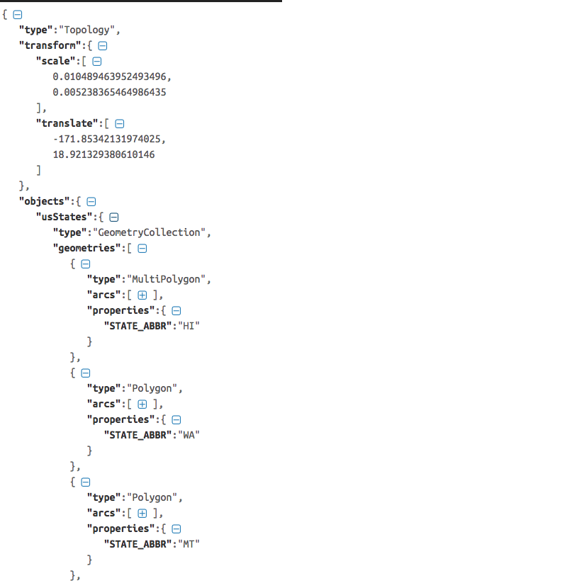
Because D3 only handles data in the GeoJSON format, there is a d3 library that does the job of converting TopoJSON to GeoJSON.

<script src="https://d3js.org/topojson.v3.js"></script>

The TopoJSON client API supports converting TopoJSON objects into GeoJSON for use in a web browser. From the documentation:

Returns the GeoJSON Feature or FeatureCollection for the specified object in the given topology. If the specified object is a GeometryCollection, a FeatureCollection is returned, and each geometry in the collection is mapped to a Feature. Otherwise, a Feature is returned. The returned feature is a shallow copy of the source object: they may share identifiers, bounding boxes, properties and coordinates.

Some examples:

A point is mapped to a feature with a geometry object of type “Point”. Likewise for line strings, polygons, and other simple geometries. A null geometry object (of type null in TopoJSON) is mapped to a feature with a null geometry object. A geometry collection of points is mapped to a feature collection of features, each with a point geometry. A geometry collection of geometry collections is mapped to a feature collection of features, each with a geometry collection.

The usage is as follows:

topojson.feature(topology, object-to-be-converted);

console.log(topojson.feature(topoJSON, topoJSON.objects.usStates))

After converting topoJSON to geoJSON, remember that what you will want to feed into the .data() portion of your d3 code, is the geoJSON.features array.

let geoJSON = topojson.feature(topoJSON,topoJSON.objects.countries);
   
...
.data(geoJSON.features) 

Using Projections

Let’s take a closer look at a GeoJSON file that contains data for the US States. Here is a data file containing US states.

{
   "type":  "FeatureCollection",
   "features":
   [
     {
       "type": "Feature",
       "id": "01",
       "properties": {"name": "Alabama"},
       "geometry": {
        "type": "Polygon",
        "coordinates": [[[-87.359296, 35.00118], [-85.606675, 34.984749], [-85.431413,34.124869],[-85.184951,32.859696], ...
 }

You can see that the coordinates are within the geometry object, and that the properties tell us that this is the shape representing Alabama.

You might be able to tell that the coordinates above use latitude and longitude - which are spherical coordinates! Mapping these onto a 2D surface like your screen in a sensible way requires a projection. There are many projections, with various advantages and disadvantages - we’ll talk about them in class.

Here is an example of how to use projections to transform lat/lon values into screen coordinate pixel values:

D3 supports a long list of projections, including:

• d3.geoAlbers - the Albers equal-area conic projection.
• d3.geoAlbersUsa - a composite Albers projection for the United States.
• d3.geoAzimuthalEqualArea - the azimuthal equal-area projection.
• d3.geoAzimuthalEquidistant - the azimuthal equidistant projection.
• d3.geoConicConformal - the conic conformal projection.
• d3.geoConicEqualArea - the conic equal-area (Albers) projection.
• d3.geoConicEquidistant - the conic equidistant projection.
• conic.parallels - set the two standard parallels.
• d3.geoEquirectangular - the equirectangular (plate carreé) projection.
• d3.geoGnomonic - the gnomonic projection.
• d3.geoMercator - the spherical Mercator projection.

You can look at the projections in more detail:

• Here is a showreel of all the projections supported by D3
• Here is an observable comparing overlap of d3 projections

Once projected to screen coordinates, the polygons can be easily converted into an SVG path with d3.geoPath(). The geoPath() function is an SVG path generator that takes in any GeoJSON feature or geometry object, and returns a formatted SVG path.

Here is a simple example of rendering the US states:

Adding markers on top of D3 Map

Now that we have the base map, we can draw marks on top of maps, in this case the size of the 50 largest cities in the US. Here are the first couple of lines of this file:

rank,place,population,lat,lon
1,New York city,8175133,40.71455,-74.007124
2,Los Angeles city,3792621,34.05349,-118.245323
3,Chicago city,2695598,45.37399,-92.888759
4,Houston city,2099451,41.337462,-75.733627

Here is an example for a choropleth map, coloring each state by its agricultural output. Here are the first couple of lines of this file:

state,value
Alabama,1.1791
Arkansas,1.3705
Arizona,1.3847
California,1.7979

The trick here is to join the data about the ouptut to the geography information: